Sample RNA-seq analysis

Downloading the data

Each of the four SRA experiments (SRX11084773, SRX11084774, SRX11084776, and SRX11084777) contains data from a single Illumina run. I used prefetch to pull down the files and then fastq-dump to convert to Gzip-compressed FastQ format.

One fun thing that happened is that I originally didn't compress the files and ran out of disk space during adapter trimming. Apparently FastQ files compress efficiently.

Describe the FastQ format

A FastQ file is a plaintext file that contains a list of sequencing reads, with each read comprising four lines¹. SRR14751157.fq contains 16,619,740 reads, so 66,478,960 lines. Here are the first four lines:

@SRR14751157.1 A00700:330:HYVGWDRXX:1:1101:25934:1000 length=100
NAATCACATCGTCATTGATGATGCTTGGGCTAGTACTGCTGCGACTTGGATCTTTCATGGTTGGTGCTCGTTGTCGTTTTTAACCCAGTGCACGGCAGCG
+SRR14751157.1 A00700:330:HYVGWDRXX:1:1101:25934:1000 length=100
#FFFFFFFFFFFFFFFFFFFFFFFFFFFFFFFFFFFFFFFFFFFFFFFFFFFFFFFFFFFFFFFFFFFFFFFFFFFFFFFFFFFFF:FF:FFFFFFF:FF

All 16,619,740 reads in the file have this same format. The line beginning with @ is the header line, beginning with the accession for the run and followed by some machine-specific metadata, ending with the length of the read (100 bases in this case). The next line is the sequence of nucleotides in the read. N represents an unknown base. The line beginning with + is a separator, and duplicates the content of the header line. The final line contains an ASCII-encoded set of quality scores for each nucleotide in the read. The quality scores indicate the level of confidence in the correctness of the nucleotide identification.

Each of these runs used single-end sequencing. With single-end sequencing, reading happens from only one end of a DNA fragment. With paired-end sequencing, reading happens from both ends of a fragment (in opposite directions). Single-end sequencing is cheaper and generates half the data of paired-end sequencing. The extra data generated by paired-end sequencing, on the other hand, allows for more accurate mapping of reads to a reference genome. This is because reading from both ends of a fragment, combined with knowledge of the distance between those two reads, enables decreased ambiguity during alignment. ^{2, 3}

Describe the biology behind the data

These data represent the transcriptome of a mouse embryonic stem cell (ESC). The RNA is synthesized from the sample and then used to generate complementary DNA (cDNA) using reverse transcription. This step is necessary because DNA sequencing is still more common than direct RNA sequencing. Two of the samples come from a wild type ESC. The other two come from an ESC that has been modified using CRISPR to knock out both alleles of the Zfp462 gene, which codes for a zinc finger protein. The experiment is performing differential gene expression analysis of the two conditions. In other words, how does gene expression change between the wild type ESC and the mutant ESC missing the target gene? The authors hypothesize that homozygous (or heterozygous) mutations of the Zfp462 gene, which is orthologous to Znf462 in humans, causes problems in neurodevelopment. They propose that Zfp462 is instrumental in a pathway that limits the accessibility of meso-endodermal gene expression sites. Without Zfp462, those expression sites are accessible, which changes cell fate specification from neural cells to meso-endodermal cells.⁴

Quality control and adapter trimming

I'm combining the QC and adapter trimming sections so I can show the charts side-by-side.

FastQC is a tool that processes FastQ files to generate high-level heuristics based on raw sequence data. Its purpose is quality control; the heuristics can be used to provide a first-pass diagnostic check before proceeding to more in-depth analyses. MultiQC combines multiple FastQC reports into a "single-pane-of-glass" dashboard. The nice thing about MultiQC is that it aggregates not just FastQC, but also other tools, like, for example, featureCounts.

FastQC provides up to 12 checks with a stop-light designation indicating "normal", "slightly abnormal", or "highly unusual" results. The red/yellow/green icons might alarm, but the documentation assures you that those results might be expected depending on your sequencing library. Maybe that means they should use a different design system, but that's out of scope for this exercise.

After an initial quality control check, I ran Trim Galore to trim adapter sequences from the data. The main reason to trim adapters prior to downstream processing is that adapters are "artificial" snippets of DNA added to the fragments under test in order to facilitate their sequencing. In other words, if you leave them in, you'll also be including irrelevant DNA that will thwart reference genome alignment and muddy up other analysis. It would be like weighing yourself while wearing a heavy winter coat, pockets full of coins and your cell phone.

Brief descriptions of the FastQC checks, along with results pre- and post-trim, follow.

Basic statistics

Per base sequence quality

Before Trimming

Summarizes and visualizes the quality scores (the fourth line of a sequence read in a FastQ file) across a given run. The X-axis is the read position. For these four runs, the read length is 100bp, so the axis runs from 0 to 100. Y-axis is quality score. Across read positions, the score for the reads across each of these samples is around 36, which is comfortably in the green.

After Trimming

Mean quality scores smoothed out and remained around 36 for all read positions.

Per tile sequence quality

Before Trimming

Another way of plotting quality scores for the sequencing data. This visualization shows quality scores by read position and flowcell tile position. It can be useful for detecting problems with the equipment (for example, if you see a cluster of low quality scores in a single region of the chart, it might indicate a problem with that region of the flowcell). The docs say "a good plot should be blue all over," and all four runs have plots that look like the Windows blue screen of death.

After Trimming

No meaningful difference.

Per sequence quality scores

Before Trimming

This third and final quality score visualization shows distribution of average quality score across reads in a given run. X-axis is average quality score for a sequence, Y-axis is number of reads with that average. Summing the Y-values (read count) over each quality score equals the total number of reads in the run.

After Trimming

No meaningful difference.

Per base sequence content

Before Trimming

Shows, across reads in a given run, the percentage of each nucleotide. FastQC wants the percentages to average out around 25% for each nucleotide, which is more or less the case for these four runs. There's some divergence near the beginning and end of reads for these runs. FastQC documentation suggests that that's not uncommon for RNA-seq, and can be explained by primers used for the reverse transcription that occurs in sequencing library preparation.

After Trimming

Ignoring the biased composition at the start of reads, the Per Base Sequence Content smoothed out considerably, and now displays a precipitous drop in %A at the end of reads—were polyA tails trimmed too?

Per sequence GC content

Before Trimming

This visualization graphs number of reads by average guanine-cytosine content (measured as a percent). In a random sequencing library, the counts should be normally distributed, and FastQC attempts to fit a normal distribution to the curve. Of the four runs, 3 errored and 1 passed. The curves all have bimodal distributions, with the first peak around 50% average GC content. Those that errored (and to a lesser extent, even the one that passed), show a spike in reads with an average GC content around 60-65%. This appears to track with the data from the previous visualization, which shows an uptick in guanine towards the end of reads.⁵

After Trimming

Distributions for each run of Per Sequence GC Content all normalized.

Per base N content

Shows the percentage of base calls at a each read position in a run for which a call can't be made, and thus is marked with an N. All four runs passed FastQC's check, showing a flatline close to 0 at all read positions.⁶

Trimming made no difference, since the N content was already at 0.

Sequence length distribution

Before Trimming

This check would show the distribution of fragment sizes (read lengths) for the run. MultiQC doesn't render a visualization here, instead showing a message that "all samples have sequences of a single length (100bp)". This can vary depending on the sequencing technology. In this case, there's no variance in sequence length.

After Trimming

After trimming, the sequences are no longer of uniform 100bp length. They now range from 20bp to 100bp. FastQC warns for files that don't have uniform read sequence lengths, hence the yellow lines in the MultiQC chart.

Sequence duplication level

Before Trimming

Visualizes sequence duplication in the library by plotting percentage of the library given to duplicates against number of duplicates in a set. For example, ~27% sequences of run SRR14751156 are paired (two copies of the sequences exist). This plot has different meanings for different kinds of sequencing. When sequencing DNA, a good library should have low levels of duplication (especially in farther along the X-axis). But when sequencing RNA, higher duplication could indicate a true biological signal, like upregulation.

After Trimming

Duplication levels didn't change drastically, although in the untrimmed sequences, about 8-12% of sequences had upwards of 10,000 duplicates; those were gone in the trimmed data. Those high range duplicates must have been the adapters.

Overrepresented sequences

This check displays a table listing reads in a run that make up more than 0.1% of the total sequences. The documentation suggests that adapter sequences may be reported in this check. For each of the runs analyzed here, the "Possible Source" column hints that the source might be the TruSeq Adapter, which is an Illumina adapter.

After trimming, no overrepresented sequences were reported in the Top Overrepresented Sequences table. This could mean that FastQC was right about the source of those outliers.

Adapter content

Before Trimming

This check uses a reference datastore of adapter Kmers to measure the percentage of adapter sequences present in a run. Charts for each of the four runs show high percentages of polyG tails. Those tails are erroneous base calls created by some Illumina sequencers, and need to be removed prior to alignment. ^{7, 8}

After Trimming

As expected, the polyG tails are now gone.

Genome mapping

Initially, I tried to run STAR on all of the FASTA files downloaded from Ensembl, but STAR warned me that I didn't have sufficient RAM to perform the genome generation. Some research in a bioinformatics forum⁹ (plus re-reading the exercise instructions) made me realize that I only needed to use the primary assembly. I deleted all FASTA files except Mus_musculus.GRCm39.dna.primary_assembly.fa.

I still had some fun with the Linux OOM killer, but eventually got my genome indexes generated. For some reason, --limitGenomeGenerateRAM didn't seem to work in my environment. --genomeSAsparseD 2 worked, but so did switching to a laptop with more RAM.¹⁰

Alignment

I used the following command to align the sample sequences to the mouse reference genome.

STAR \
    --runThreadN 16 \
    --genomeDir genome-indexes \
    --outFileNamePrefix ./alignment/ \
    --readFilesCommand zcat \
    --readFilesIn data-trimmed/SRR14751156_trimmed.fq.gz,data-trimmed/SRR14751157_trimmed.fq.gz,data-trimmed/SRR14751159_trimmed.fq.gz,data-trimmed/SRR14751160_trimmed.fq.gz \
    --outSAMattrRGline ID:WT_Rep1 , ID:WT_Rep2 , ID:MUT_Rep1 , ID:MUT_Rep2

I didn't get too fancy with the command-line arguments, preferring to start with the defaults and see how far that gets me.

• --runThreadN parallelizes the process across 16 CPU cores.
• --genomeDir and --outFileNamePrefix specify options for input and output locations.
• --readFilesCommand zcat allows STAR to operate on Gzip-compressed FastQ files.
• --readFilesIn specifies the sample data to align to the reference genome in a comma-separated list of FastQ files.

--outSAMattrRGline is the fanciest I got. It took some time for me to realize I needed that flag. When running featureCounts, I couldn't figure out how to group counts by sample. They were all showing up in one aggregate column. Reading documentation, I finally learned that you use the --byReadGroup option in featureCounts to prevent aggregating across samples. But you also have to include read group annotations in the alignment file, which is accomplished with the --outSAMattrRGline option. Combining that flag with the featureCounts flag was a breakthrough.

Transcripts quantification

I ran the following command to summarize read counts by gene meta-feature. By default, featureCounts summarizes by meta-feature (gene), rather than feature (exon). It also discards reads that map to multiple meta-features by default.¹¹

featureCounts \
    alignment/Aligned.out.sam \
    -a Mus_musculus.GRCm39.111.gtf \
    -G Mus_musculus.GRCm39.dna.primary_assembly.fa \
    -J \
    -o counts/counts.txt \
    -T 16 \
    --byReadGroup \
    --extraAttributes gene_name

• -a and -o specify mandatory input and output options (for the annotations files and the read counts matrix, respectively).
• -G and -J combine to improve counts for meta-feature reads that span exon splice junctions.
• -T spreads the computation across multiple CPU cores for performance improvement.
• As discussed above, --byReadGroup aggregates read counts by sample. For the experiment, it resulted in four data columns in the read counts matrix, showing read counts for genes in each sample.
• --extraAttributes gene_name adds a column for the gene name (e.g., Zfp462), pulled from the annotations file. Including this in the matrix makes downstream processing and visualization much nicer, since you get to see gene names instead of gene IDs.

Downstream processing

Pre-filtering

The purpose of pre-filtering is to discard rows from the DESeqDataSet that have counts too low to be meaningful or of interest for analysis. It can speed up the DESeq2 model and decrease memory usage. It also improves visualizations by filtering out the noise of genes with no information. For example, in this counts matrix, 68% of genes in the table have a count of 0 across all four samples.

> nrow(dds[(rowSums(counts(dds) == 0)),]) / nrow(dds)
[1] 0.6823889

The DESeq2 documentation suggests filtering out genes with a read count below 10 for the purposes of RNA-seq. Their recommendation for filtering criteria is to filter out any genes where there are fewer than n samples with at least 10 reads, where n is the size of the smallest sample group. In this analysis, each group has two samples, so

This cuts the number of rows in the table from 57,180 to 14,812.

Assess mean-variance relationship

Following Love et al, I decided to use meanSdPlot from vsn for these plots.¹² Mean-variance plots graph the variability of gene counts across the samples against the average counts for those genes. They can be used for quality control, ensuring that variances don't get too high (which could indicate a problem with the underlying data) and they can also indicate possible genes of interest. Those with high variances could point to a biologically significant difference in gene expression from one condition to the other.

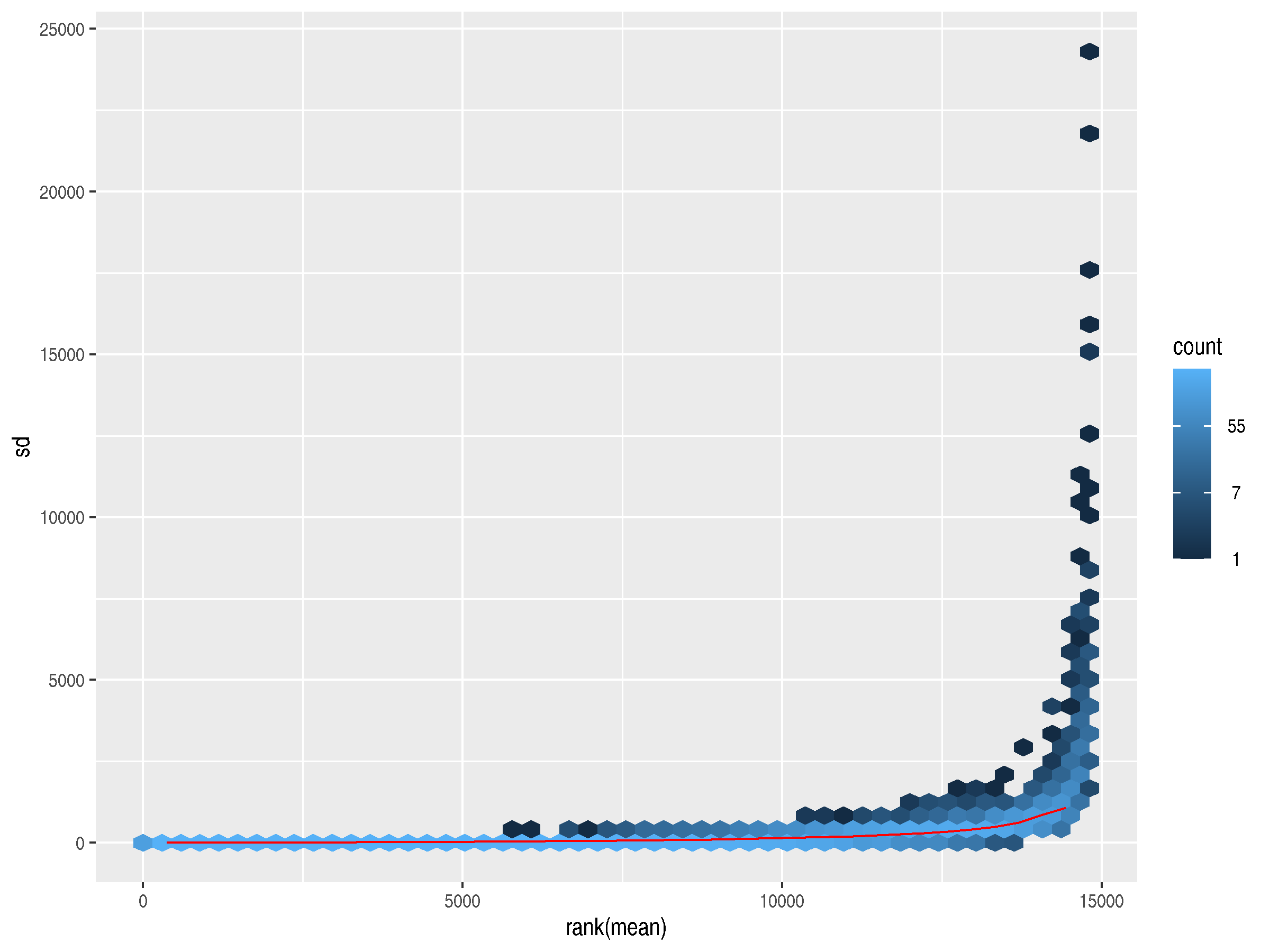
The plot generated from the raw counts shows a slight trend upward in variance as the mean increases. The highly expressed genes have much higher standard deviations, so they dominate the plot.

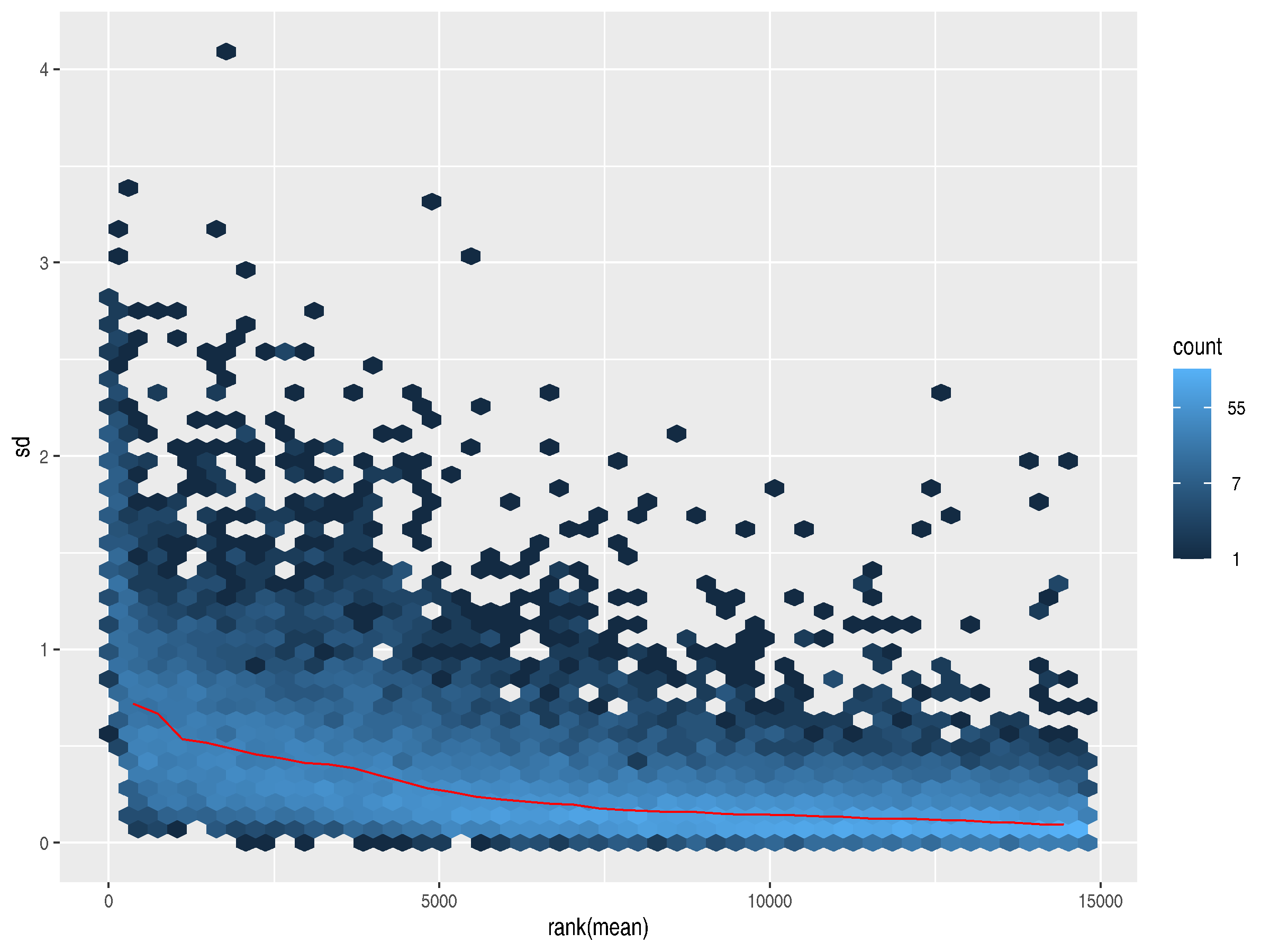
A standard log₂ transformation can address the dominance of the highly variable, highly expressed genes, but it over-corrects, inverting the relationship. Now, lowly expressed genes have slightly higher standard deviations.

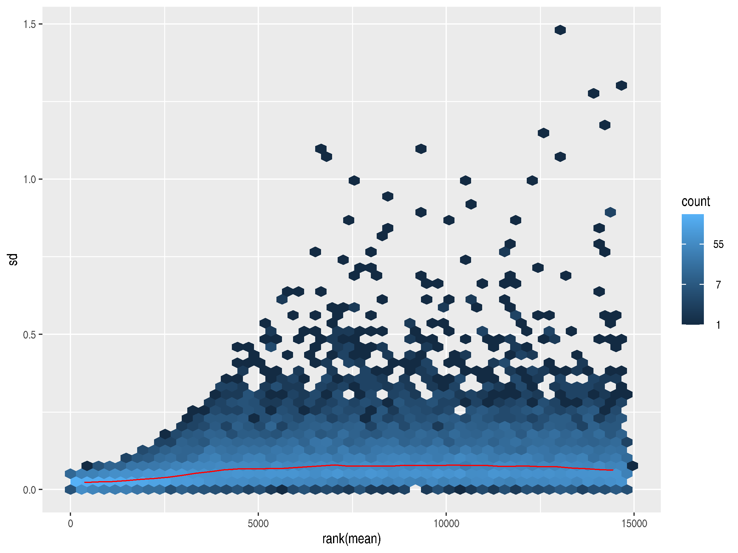
To address both these problems, the authors of DESeq2 provide rlog, which differentially treats genes at either end of the expression counts spectrum. Here, the trend line flattens out, indicating a lack of dependence of the variance on the mean. Removing the dependence allows for an accurate plotting of the variances for outlier detection and quality control.

Principal component analysis (PCA)

PCA is used for sample clustering analysis. It uses the gene counts per sample to generate principal component axes and then plots each sample on the axes. Samples that cluster together are more closely related. For this analysis, clustered samples mean that the gene expression activity is similar in those sample groups.

In this experiment, the wild type samples clustered on one side of PC1 and the mutant Zfp462 knockout samples clustered on the other side, as expected. Interesting to note that PC1 was responsible for virtually all the variance in the samples.

DESeq2

I ran DESeq like this:¹³

About 58% of the genes in the results table had adjusted P values above 0.1, and I filtered them out. Then I generated a bar plot counting the number of upregulated and downregulated genes. For my own curiosity, I also created a bar plot showing the log₂ fold-change for the top 10 upregulated and top 10 down regulated genes.

And finally, a Volcano plot plotting effect-size against fold-change. You can hover, and drag to zoom.